Understanding SQN Metrics at Quants Space

Standard SQN and Adjustments for Trading Frequency and Position Size

At Quants Space, we include several System Quality Number (SQN) metrics in our strategy performance reports. They compare average position ROI with its variability and adjust for the number of positions. We show multiple variants because strategies with similar returns per position can trade at very different frequencies and with different position sizes. This guide explains where SQN comes from, how we calculate our metrics and how to interpret them.

Where SQN Comes From

Trading educator Van K. Tharp developed SQN while studying the relationship between trading-system quality and position sizing. His original framework expresses each completed trade as an R-multiple: profit or loss divided by the amount initially risked. A gain of $200 on an initial risk of $100 is +2R; a loss of $100 is -1R. The average R-multiple is the system's expectancy.

Tharp's SQN combines that expectancy with the standard deviation of the R-multiple distribution and the square root of the number of closed trades. It summarizes the consistency of trade results and the number of observations; it does not guarantee a particular return or drawdown.

$$\mathrm{SQN}=\frac{\bar R}{\sigma_R}\sqrt{N}$$

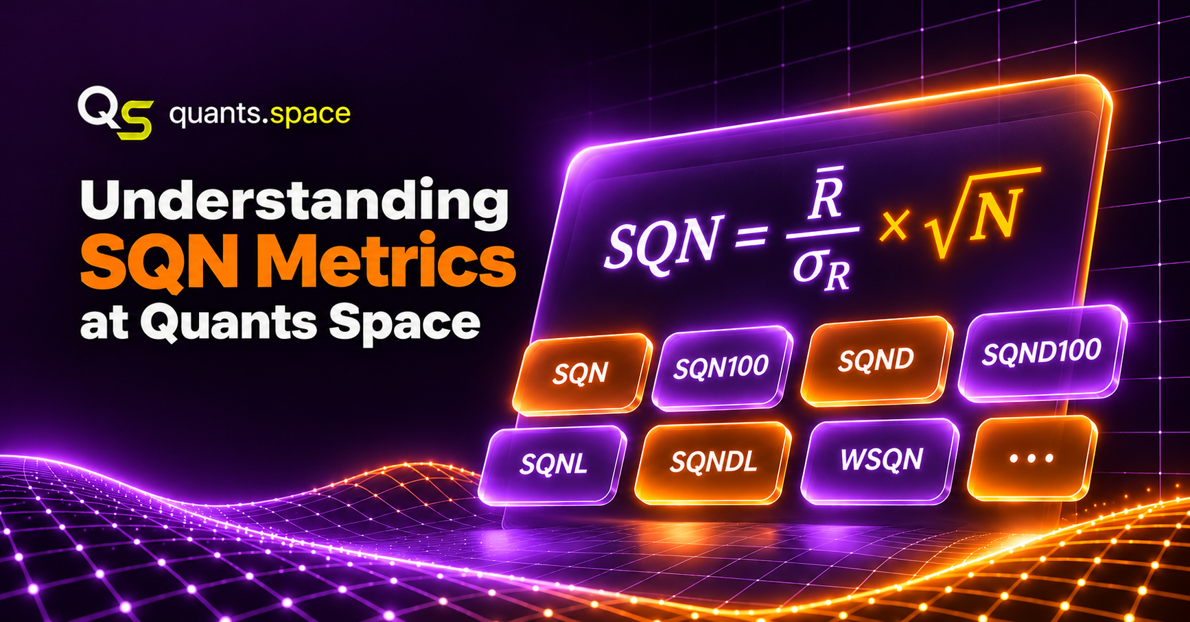
Here, N is the number of closed trades, R-bar is the mean R-multiple, and the denominator is the standard deviation of the R-multiples. In Quants Space reports, we use position ROI instead of R-multiples. Because these measure different kinds of returns, their SQN values are comparable only when the calculation methods match.

SQN Calculation in Five Trades

Suppose each trade risks $100 and the completed results are +1R, +2R, -1R, +2R and +1R. The five trades earn a total of +5R.

Trade	Profit or loss	R-multiple
1	+$100	+1R
2	+$200	+2R
3	-$100	-1R
4	+$200	+2R
5	+$100	+1R

$$\bar R=\frac{(+1)+(+2)+(-1)+(+2)+(+1)}{5}=+1.00\mathrm{R}$$

The squared deviations from the +1R mean are 0, 1, 4, 1 and 0. The -1R trade, for example, is 2R below the mean; squaring -2 gives 4. Their sum is 6:

$$\sigma_R=\sqrt{\frac{0+1+4+1+0}{5}}=\sqrt{\frac{6}{5}}=1.0954$$

Substituting into the SQN formula:

$$\mathrm{SQN}=\frac{1.00}{1.0954}\sqrt{5}=2.04$$

The score is 2.04. This five-trade example demonstrates the SQN calculation; evaluating a strategy requires many more trades and representative market conditions.

Why Trading Frequency Matters

Raw SQN does not use a fixed calendar period. If average ROI and its standard deviation stay constant, multiplying the number of positions by ten increases SQN by the square root of ten. A strategy that trades more often can therefore show a much larger raw SQN than one with the same returns per position but fewer trades.

Measure	Strategy A	Strategy B
Average R-multiple	0.20	0.20
R-multiple standard deviation	1.00	1.00
Trades per year	100	1,000
Years tested	5	5
Total trades	500	5,000
Raw SQN	4.47	14.14
SQN with trade-count scaling capped at 100	2.00	2.00
Illustrative SQN using trades per year	2.00	6.32

Capping the scaling count at 100 reduces the effect of total trade count, but every trade still contributes to the mean and standard deviation. The trades-per-year example illustrates annual trading frequency; it is not a Quants Space metric. Neither adjustment captures correlated or overlapping trades, transaction costs or capacity limits. We still need daily portfolio returns to assess portfolio risk.

$$\mathrm{SQN}_{100}=\frac{\bar R}{\sigma_R}\sqrt{\min(N,100)}$$

SQN Metrics in Our Performance Reports

In Quants Space reports, SQN is mean position ROI divided by its standard deviation, multiplied by the square root of the number of positions. Other variants change the position-count scaling factor or weight returns by position size. This helps readers distinguish consistency of returns from trading frequency and position sizing.

Report metric	Meaning of the adjustment
SQN	Uses the square root of total position count
SQN100	Limits the position count used for scaling to 100
SQND	Uses average positions per day for scaling
SQND100	Limits the daily position count used for scaling to 100
SQNL	Uses log10 of total positions with a minimum input of 1
SQNDL	Uses log10 of average positions per day with a minimum input of 1
W-prefixed metrics	Uses position-size-weighted ROI statistics

Our L variants multiply mean ROI divided by its standard deviation directly by log10(max(position count, 1)); no square root is applied. For example, log10(1) = 0, log10(100) = 2 and log10(1,000) = 3. Other variants use sqrt(position count). Daily variants use average positions per day, not portfolio returns, and are not annualized Sharpe ratios.

Position-Size-Weighted SQN Example

At Quants Space, position size determines the weight of each ROI. Our weighted_mean(values, weights) calculates sum(values * weights) / sum(weights). We calculate weighted standard deviation by taking the square root of the position-size-weighted mean of squared ROI deviations. In the formulas, s_i is position size and r_i is ROI:

$$\mu_w=\frac{\sum_i s_i r_i}{\sum_i s_i}$$ $$\sigma_w=\sqrt{\frac{\sum_i s_i(r_i-\mu_w)^2}{\sum_i s_i}}$$

Consider four illustrative positions opened over two days:

Position	Day	Position size	ROI	Profit or loss	Weight
1	Day 1	$1,000	+2%	+$20	10%
2	Day 1	$1,000	+2%	+$20	10%
3	Day 2	$4,000	-1%	-$40	40%
4	Day 2	$4,000	+1%	+$40	40%

We use the same four ROI observations for SQN and WSQN, but calculate their means and standard deviations separately because weighting changes the contribution of each position.

Unweighted SQN. First, each position contributes equally to the mean ROI:

$$\bar r=\frac{2+2-1+1}{4}=1.00\%$$

The deviations are 1, 1, -2 and 0 percentage points. Their standard deviation is:

$$\sigma=\sqrt{\frac{1^2+1^2+(-2)^2+0^2}{4}}=\sqrt{1.50}=1.2247\%$$ $$\mathrm{SQN}=\frac{1.00}{1.2247}\sqrt{4}=1.6330$$

Position-size-weighted SQN. Now each position contributes according to its position size:

$$\mu_w=\frac{1000(2)+1000(2)+4000(-1)+4000(1)}{10000}=0.40\%$$

The deviations from the weighted mean of 0.40% are 1.6, 1.6, -1.4 and 0.6 percentage points. We apply the same position sizes to the squared deviations:

$$\sigma_w=\sqrt{\frac{1000(1.6)^2+1000(1.6)^2+4000(-1.4)^2+4000(0.6)^2}{10000}}$$ $$\sigma_w=\sqrt{\frac{2560+2560+7840+1440}{10000}}=\sqrt{1.44}=1.20\%$$ $$\mathrm{WSQN}=\frac{0.40}{1.20}\sqrt{4}=0.6667$$

The results differ because the larger positions in this example have less favorable returns.

We can apply all 12 SQN variants to these same positions. The four positions were opened over two days, giving an average of two positions per day. The unweighted mean-to-standard-deviation ratio is 1.00 / 1.2247 = 0.8165, and the position-size-weighted ratio is 0.40 / 1.20 = 0.3333. We multiply each ratio by the same position-count scaling factor to obtain the unweighted and weighted variants.

Variant pair	Scaling factor	Unweighted	Position-size weighted
SQN / WSQN	sqrt(4) = 2.0000	1.6330	0.6667
SQN100 / WSQN100	sqrt(min(4,100)) = 2.0000	1.6330	0.6667
SQND / WSQND	sqrt(2) = 1.4142	1.1547	0.4714
SQND100 / WSQND100	sqrt(min(2,100)) = 1.4142	1.1547	0.4714
SQNL / WSQNL	log10(4) = 0.6021	0.4916	0.2007
SQNDL / WSQNDL	log10(2) = 0.3010	0.2458	0.1003

Because both position counts are below 100, the capped variants equal their uncapped counterparts. The logarithmic variants use log10(4) = 0.6021 or log10(2) = 0.3010 directly, without a square root. These small counts illustrate the formulas; they are not enough to judge a trading strategy.

Pros and Cons of Our SQN Metrics

We offer several SQN variants because each adjustment to position count answers a different question. These scores help compare strategies, but none alone establishes future profitability, trade independence or acceptable portfolio risk.

Method	Main advantage	Main limitation
Raw SQN	Combines mean position ROI, its standard deviation and position count.	Increases with sqrt(N), even if position outcomes are unchanged. Correlated positions weaken its interpretation.
SQN100	Reduces the advantage of very large position counts when comparing backtests.	The limit of 100 is a chosen threshold. More positions do not increase the scaling factor after that point.
SQND and SQND100	Shows the effect of average positions traded per day.	Trades per day can still vary greatly between high-frequency and low- or medium-frequency strategies, so SQND remains frequency-sensitive. SQND100 caps the count at 100 per day.
SQNL and SQNDL	Base-10 logarithms reduce the influence of very high position counts.	The minimum input of 1 prevents negative log factors, but log10(1) = 0, so low-frequency differences can disappear.
Weighted variants	Shows whether larger positions have returns as consistent as smaller ones.	A few large positions can dominate weighted statistics. Position size does not capture risk or holding period.

How We Recommend Reading the Metrics

We recommend comparing strategies over similar backtest periods and using consistent ROI definitions and position-count rules. Review SQN alongside net ROI, transaction costs, turnover, daily portfolio returns, Sharpe ratio, drawdown and exposure. Pay particular attention to overlapping positions and strategies selected from many tested configurations: strong backtest results do not guarantee out-of-sample performance.